Priority Queue Applications: Heap Sort and Dijkstra's Algorithm

About This Module

This module explores two major applications of priority queues: heap sort for efficient sorting and Dijkstra's algorithm for finding shortest paths in weighted graphs. We'll implement both algorithms using Rust's BinaryHeap and analyze their performance characteristics.

Prework

Prework Reading

Read the following sections from "The Rust Programming Language" book:

Chapter 8.1: Storing Lists of Values with Vectors
Chapter 8.3: Storing Keys with Associated Values in Hash Maps
Review BinaryHeap documentation and priority queue concepts

Pre-lecture Reflections

Before class, consider these questions:

How does heap sort compare to other O(n log n) sorting algorithms in terms of space complexity?
Why is Dijkstra's algorithm considered a greedy algorithm, and when does this approach work?
What are the limitations of Dijkstra's algorithm with negative edge weights?
How do priority queues enable efficient implementation of graph algorithms?
What are the trade-offs between different shortest path algorithms?

Lecture

Learning Objectives

By the end of this module, you should be able to:

Implement heap sort using priority queues and analyze its complexity
Understand and implement Dijkstra's shortest path algorithm
Use Rust's BinaryHeap for efficient priority-based operations
Compare heap sort with other sorting algorithms
Design graph representations suitable for shortest path algorithms
Analyze time and space complexity of priority queue applications

Application 1: Sorting a.k.a. HeapSort

Put everything into a priority queue
Remove items in order

#![allow(unused)]
fn main() {
use std::collections::BinaryHeap;

fn heap_sort(v:&mut Vec<i32>) {
    let mut pq = BinaryHeap::new();
    for v in v.iter() {
        pq.push(*v);
    }

    // to sort smallest to largest we iterate in reverse
    for i in (0..v.len()).rev() {
        v[i] = pq.pop().unwrap();
    }
}
}

#![allow(unused)]
fn main() {
let mut v = vec![23,12,-11,-9,7,37,14,11];
heap_sort(&mut v);
v
}

[-11, -9, 7, 11, 12, 14, 23, 37]

Total running time: $O (n lo g n)$ for $n$ numbers

More direct, using Rust operations

#![allow(unused)]
fn main() {
fn heap_sort_2(v:Vec<i32>) -> Vec<i32> {
   BinaryHeap::from(v).into_sorted_vec()
}
}

No extra memory allocated: the initial vector, intermediate binary heap, and final vector all use the same space on the heap

BinaryHeap::from(v) consumes v
into_sorted_vec() consumes the intermediate binary heap

#![allow(unused)]
fn main() {
let mut v = vec![7,17,3,1,8,11];
heap_sort_2(v)
}

[1, 3, 7, 8, 11, 17]

Sorting already provided for vectors (currently use other algorithms): sort and sort_unstable

HeapSort is faster in time, but takes twice the memory.

#![allow(unused)]
fn main() {
let mut v = vec![7,17,3,1,8,11];
v.sort();
v
}

[1, 3, 7, 8, 11, 17]

#![allow(unused)]
fn main() {
let mut v = vec![7,17,3,1,8,11];
v.sort_unstable(); // doesn't preserve order for equal elements
v
}

[1, 3, 7, 8, 11, 17]

Application 2: Shortest weighted paths (Dijkstra's algorithm)

Input graph: edges with positive values, directed or undirected
Edge is now (starting node, ending node, cost)
Goal: Compute all distances from a given vertex $v$

Some quotes from Edsger Dijkstra

Pioneer in computer science. Very opinionated.

The use of COBOL cripples the mind; its teaching should, therefore, be regarded as a criminal offence.

It is practically impossible to teach good programming to students that have had a prior exposure to BASIC: as potential programmers they are mentally mutilated beyond hope of regeneration.

One morning I was shopping in Amsterdam with my young fiancée, and tired, we sat down on the café terrace to drink a cup of coffee and I was just thinking... Eventually, that algorithm became to my great amazement, one of the cornerstones of my fame

Shortest Weighted Path Description

Mark all nodes unvisited. Create a set of all the unvisited nodes called the unvisited set.
Assign to every node a tentative distance value:
1. set it to zero for our initial node and to infinity for all other nodes.
2. During the run of the algorithm, the tentative distance of a node v is the length of the shortest path discovered so far between the node v and the starting node.
3. Since initially no path is known to any other vertex than the source itself (which is a path of length zero), all other tentative distances are initially set to infinity.
4. Set the initial node as current.
For the current node, consider all of its unvisited neighbors and calculate their tentative distances through the current node.
1. Compare the newly calculated tentative distance to the one currently assigned to the neighbor and assign it the smaller one.
2. For example, if the current node A is marked with a distance of 6, and the edge connecting it with a neighbor B has length 2, then the distance to B through A will be 6 + 2 = 8.
3. If B was previously marked with a distance greater than 8 then change it to 8. Otherwise, the current value will be kept.
When we are done considering all of the unvisited neighbors of the current node, mark the current node as visited and remove it from the unvisited set.
1. A visited node will never be checked again
2. (this is valid and optimal in connection with the behavior in step 6.: that the next nodes to visit will always be in the order of 'smallest distance from initial node first' so any visits after would have a greater distance).
If all nodes have been marked visited or if the smallest tentative distance among the nodes in the unvisited set is infinity (when planning a complete traversal; occurs when there is no connection between the initial node and remaining unvisited nodes), then stop. The algorithm has finished.
Otherwise, select the unvisited node that is marked with the smallest tentative distance, set it as the new current node, and go back to step 3.

How it works:

Greedily take the closest unprocessed vertex
- Its distance must be correct
Keep updating distances of unprocessed vertices

Example

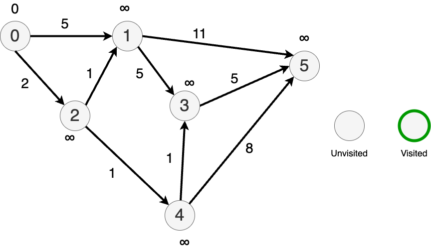
Let's illustrate by way of example: Directed graph with weighted edges.

Pick 0 as a starting node and assign it's distance as 0.

Assign distance of $\infty$ to all other nodes.

From 0, travel to each connected node and update the tentative distances.

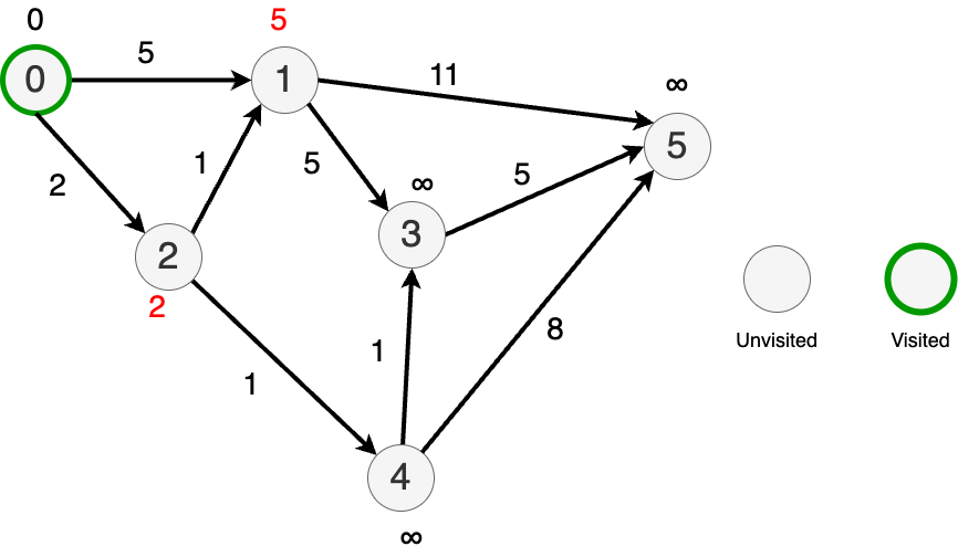
Now go to the "closest" node (node 2) and update the distances to its immediate neighbors.

Mark node 2 as visited.

Randomly pick between nodes 4 and 1 since they both have updated distances 3.

Pick node 1.

Update the distances to it's nearest neighbors.

Mark node 1 as visited.

Now, pick the node with the lost distance (node 4) and update the distances to it's nearest neighbors.

Distances to nodes 3 and 4 improved.

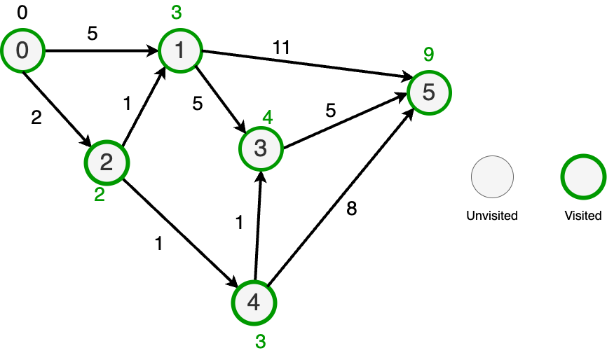
Then, go to node 3 and update its distance to its nearest neighbor.

Nowhere else to go so mark everything as done.

BinaryHeap to the rescue

Since we always want to pick the cheapest node, we can use a BinaryHeap to find the next node to check.

Dijkstra's Shortest Path Implementation

Auxiliary graph definitions

#![allow(unused)]
fn main() {
use std::collections::BinaryHeap;

type Vertex = usize;
type Distance = usize;
type Edge = (Vertex, Vertex, Distance);  // Updated edge definition.

#[derive(Debug,Copy,Clone)]
struct Outedge {
    vertex: Vertex,
    length: Distance,
}

type AdjacencyList = Vec<Outedge>;   // Adjacency list of Outedge's

#[derive(Debug)]
struct Graph {
    n: usize,
    outedges: Vec<AdjacencyList>,
}

impl Graph {
    fn create_directed(n:usize,edges:&Vec<Edge>) -> Graph {
        let mut outedges = vec![vec![];n];
        for (u, v, length) in edges {
            outedges[*u].push(Outedge{vertex: *v, length: *length});  // 
        }
        Graph{n,outedges}
    }
}
}

Load our graph

#![allow(unused)]
fn main() {
let n = 6;
let edges: Vec<Edge> = vec![(0,1,5),(0,2,2),(2,1,1),(2,4,1),(1,3,5),(4,3,1),(1,5,11),(3,5,5),(4,5,8)];
let graph = Graph::create_directed(n, &edges);
graph
}

Graph { n: 6, outedges: [[Outedge { vertex: 1, length: 5 }, Outedge { vertex: 2, length: 2 }], [Outedge { vertex: 3, length: 5 }, Outedge { vertex: 5, length: 11 }], [Outedge { vertex: 1, length: 1 }, Outedge { vertex: 4, length: 1 }], [Outedge { vertex: 5, length: 5 }], [Outedge { vertex: 3, length: 1 }, Outedge { vertex: 5, length: 8 }], []] }

Our implementation

#![allow(unused)]
fn main() {
let start: Vertex = 0;

let mut distances: Vec<Option<Distance> > = vec![None; graph.n];  // use None instead of infinity
distances[start] = Some(0);
}

#![allow(unused)]
fn main() {
use core::cmp::Reverse;

let mut pq = BinaryHeap::<Reverse<(Distance,Vertex)>>::new();  // make a min-heap with Reverse
pq.push(Reverse((0,start)));
}

#![allow(unused)]

fn main() {
// loop while we can pop -- deconstruct
while let Some(Reverse((dist,v))) = pq.pop() { // boolean, not assignment
    
    for Outedge{vertex,length} in graph.outedges[v].iter() {
        
        let new_dist = dist + *length;

        
        let update = match distances[*vertex] { // assignment match
            None => {true}
            Some(d) => {new_dist < d}
        };

        // update the distance of the node
        if update {
            distances[*vertex] = Some(new_dist);  // record the new distance
            pq.push(Reverse((new_dist,*vertex)));
        }
    }
};
}

#![allow(unused)]
fn main() {
distances
}

[Some(0), Some(3), Some(2), Some(4), Some(3), Some(9)]

Complexity and properties of Dijkstra's algorithm

$O (V^{2})$ -- worst case visit (N-1) nodes on every node
Works just as well with undirected graphs
Doesn't work if path weights can be negative (why?)

Traveling salesman

On the surface similar to shortest paths

Given an undirected graph with weighted non-negative edges find the shortest path that starts at a specified vertex, traverses every vertex in the graph and returns to the starting point.

Applications:

Amazon deliver route optimization
Drilling holes in circuit boards -- minimize stepping motor travel.

DS210 Course Notes